2.3 Closed form solution of the estimated parameters
We define the diagonal matrix  containing part of the coefficients of the power series as shown in (
6
).
containing part of the coefficients of the power series as shown in (
6
).

 | (6) |
In addition, we define the  -element column vector
  shown in (
7
) that contains powers of the scalar real parameter
shown in (
7
) that contains powers of the scalar real parameter  ,
,  .
.
 | (7) |
Using (
5
), (
6
) and (
7
), we can rewrite  as shown in (
8
).
as shown in (
8
).
 | (8) |
Premultiplying by the least-squares idempotent matrix  yields the residuals
  , allowing us to express the overall sum-of-squared errors as in (
9
),
, allowing us to express the overall sum-of-squared errors as in (
9
),
 | (9) |
where 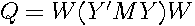 . The matrix
  represents residuals from regressing the dependent variable and the spatial lags of the dependent variable on the independent variables
  . Multiplying by a vector
  results in a linear combination of these residuals,
  . Hence, the sum-of-squared errors associated with this vector equals
  . If a linear combination of the residuals, produces a zero vector (columns of are not linearly independent), then
 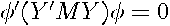 and
and  is positive semidefinite in this case, since the product cannot be negative. This seems unlikely to arise in practice, so we assume the regression residuals are linearly independent so that is nonsingular. In this case,
 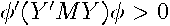 and
and  is positive definite. Given this, both and are symmetric positive definite matrices, so
  must be congruent to and have the same number of positive eigenvalues as by Sylvester’s law of inertia (Strang(1976, p. 246)). Since is a symmetric positive definite matrix, will have all positive eigenvalues and must be a symmetric positive definite matrix (Horn and Johnson (1993), p. 402).
The overall sum-of-squared errors  is a
is a  degree polynomial in the variable . The coefficients in the polynomial are the sum of all terms appearing in associated with each power of . The number of coefficients of a degree polynomial equals
  due to the constant term (coefficient associated with the degree 0). Specifically, the coefficients
  , a element column vector are shown in (
10
),
, a element column vector are shown in (
10
),
 | (10) |
where  is an indicator function taking on values of 1 when the condition is true. The terms associated with the same power of have subscripts
  that sum to the same value. For example,
 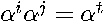 when
when  , which means that each coefficient
  is the sum of the elements along the antidiagonals of . This allows us to rewrite as the degree polynomial
  , shown in (
11
).
, shown in (
11
).
 | (11) |
To find the minimum of the sum-of-squared errors, we differentiate the polynomial in (
11
) with respect to , equate to zero, and solve for as shown in (
12
).
 | (12) |
The derivative  is a degree
  polynomial and thus has possible roots. The problem of finding all the roots of a polynomial has a well-defined solution. Specifically, the roots equal the eigenvalues of the companion matrix associated with the polynomial (Horn and Johnson (1993, p. 146-147)).
 Computation of the eigenvalues requires
  operations in this case and does not depend upon
  . Thus, the maximum likelihood estimates have a closed-form solution in terms of the eigenvalues of a small matrix.

 Other methods also exist for finding the roots of polynomials. See Press et al. (1996, p. 362-372) for a review of these.
