Quick Computation of Spatial Autoregressive Estimators
By
R. Kelley Pace
LREC Chair of Real Estate
E.J. Ourso College of Business
Louisiana State University
Baton Rouge, LA 70803-6308
(578)-388-6256
and
Ronald Barry
Associate Professor of Mathematical Sciences
University of Alaska
Fairbanks, Alaska 99775-6660
(907)-474-7226
FAX: (907)-474-5394
FFRPB@aurora.alaska.edu
The contact information is updated from the published manuscript.
This was published in:
Pace, R. Kelley, and Ronald Barry, “Quick Computation of Regressions with a Spatially Autoregressive Dependent Variable,” Geographical Analysis, Volume 29, Number 3, July 1997, p. 232-247.
We would like to thank Ohio State University Press for having granted us copyright permission to distribute this electronic version of the paper. Ohio State University Press owns the copyright to this work.
Abstract:
Spatial estimators usually require the manipulation of n2 relations among n observations and use operations such as determinants, eigenvalues, and inverses whose operation counts grow at a rate proportional to n3. This paper provides ways to quickly compute estimates when the dependent variable follows a spatial autoregressive process, which by appropriate specification of the independent variables can subsume the case when the errors follow a spatial autoregressive process. Since only nearby observations tend to affect a given observation, most observations have no effect and hence the spatial weight matrix becomes sparse. By exploiting sparsity and rearranging computations, one can compute estimates at low cost. As a demonstration of the efficacy of these techniques, the paper provides a Monte Carlo study whereby 3107 observation regressions require only 0.1 seconds each when using Matlab on a 200Mhz Pentium Pro personal computer. In addition, the paper illustrates these techniques by examining voting behavior across US counties in the 1980 presidential election.
ACKNOWLEDGMENTS:
We would like to thank the University of Alaska for its generous research support. In particular, we would like to thank Todd Lee for his comments. In addition, Pace would like to thank the Center for Real Estate and Urban Economics, University of Connecticut for its support. We would both like to thank the referees and the editor for their careful reading of the manuscript and the resultant suggestions which have led to considerable improvements.
Quick Computation of Spatial Autoregressive Estimators
Introduction
The examination of empirical data over space, with explicit recognition of the influence each observation has upon the others, has made large gains since the seminal contributions of Whittle (1954). For example, Ord (1975) proposed an algorithm involving eigenvalues which made spatial estimation practical for small to moderate sized data sets. In addition, Griffith (1988), Anselin (1988), Haining (1990), Anselin and Hudak (1992), and others have worked on the implementation of spatial estimation and have provided actual code in major languages for computing spatial estimates.
Despite these advances much work needs to be done to extend the benefits of spatial estimation to larger data sets made increasingly available by the widespread use of geographic information systems. Spatial estimators by necessity must examine the relation between each observation and every other observation. This leads to the use of n by n matrices where n represents the number of observations. Quickly, the logistics spiral out-of-control: a 10,000 observation problem creates a 10,000 by 10,000 matrix which would require 800MB of storage (double precision). Computational counts for operations such as determinants and inverses grow with the cube of n. Point estimates alone create these computational exigencies — inference can further exacerbate the computational demands.
As an additional problem, traditional maximum likelihood techniques require non-linear optimization techniques using either analytic derivatives or finite difference approximations. Unfortunately, these can fail to find the global optimum and do so without informing the user of their failure. For example, Ripley (1988, p. 11-15) provides an example with numerous local optima in a one-parameter profile likelihood problem.
Hence, an ideal spatial estimator would (a) handle large data sets; (b) handle point estimation and inference quickly; and (c) not rely on local non-linear optimization algorithms. This paper provides algorithms which achieve all of these goals.
The main weapon against these problems is sparseness, the prevalence of zeros in a matrix. The zeros arise because only nearby observations directly affect each other. Sparseness greatly accelerates computations and reduces storage requirements. For example, sparseness allows us to compute 100 determinants of 3107 by 3107 matrices in 83 seconds. Moreover, while the dense version of these matrices would require 77MB, the sparse version requires less than 1MB. A secondary method is based on reorganizing the computations in the likelihood to avoid iteration and to solve equations as opposed to computing inverses.
We examine the case where the dependent variable follows a spatial autoregressive process. This case can subsume the autoregressive process in errors case when the independent variables include variables with their spatial lags (Anselin 1988, p. 227).
To illustrate our technique, we provide an example and a simulation using U.S. counties or their equivalents. Counties have many attractive characteristics as a geographical entity. First, they tend to have stable definitions over recent time in contrast to census tracts and blocks. Second, many variables are available at this level of aggregation. For example, USA Counties on CD-ROM contains 2,844 variables across 3,141 counties or their equivalents across the U.S. These data cover many topics of interest such as age, agriculture, crime, housing, income, education, and elections. More aggregation would destroy the geographical nature of the data and less aggregation often reduces data availability because of problems with ensuring the privacy of respondents.
As our empirical example, we model voting behavior across space. Many countries have automatic voter registration and compulsory voter turnout. In contrast, the relatively low rate of voter registration and turnout in the U.S. generates considerable comment. Most of the discussion centers around variables such as income, traditionally discussed without explicitly considering spatial effects. However, political offices and parties have traditionally been organized in hierarchies using such geographical entities as precincts, wards, counties, and states. It seems plausible that the effects of voting across space cannot be completely described by a small number of observable independent variables. To what degree do the observable independent variables versus the spatial effects describe voting behavior across US counties? We show how our techniques facilitate investigating the question of the relative importance of these two components.
In addition, we conduct a Monte Carlo experiment involving 22,500 regressions of 3107 observations per regression using the same spatial weight matrix employed in the empirical voting example. The simulation demonstrates how sparsity greatly reduces the difficulty of generating vectors of spatially dependent variates. As we show, it takes, on average, only 0.1 second each using the Matlab language on a 200Mhz Pentium Pro to generate a spatially dependent vector and to find the resultant estimates.
The next section presents the model, likelihood function, and estimation procedures. Latter sections show the role of sparsity, illustrate the techniques with a voting example, and discuss a Monte Carlo study of the estimator. The final section presents the key results.
A Quick Spatial Autoregressive Estimator
This overall section discusses estimation of a spatial autoregressive process in the dependent variable. Part 1 presents the model and its likelihood, part 2 discusses the estimated generalized least squares (EGLS) and maximum likelihood (ML) estimation of the model, while part 3 provides a means to conduct inference without computing information matrices, and part 4 examines the computation of likelihood ratio tests.
1. The Spatial Autoregressive Likelihood Function
When the dependent variable exhibits spatial autocorrelation, the simultaneous
autoregression estimator corrects the usual prediction of the dependent variable,
![]() , by a weighted average of the values on nearby observations, DY.
, by a weighted average of the values on nearby observations, DY.
![]()
()1
where D represents an n by n weighting matrix with 0s on the
diagonal (the observation cannot predict itself) and ![]() represents
the autoregressive parameter. We could also rewrite as .
represents
the autoregressive parameter. We could also rewrite as .
![]()
()2
Hence, we are looking for some optimal convex combination of Y in levels and its spatial first differences (I-D)Y. To maintain the interpretation of a weighted average, the rows of D sum to 1 as implied by below. Such weighting matrices are said to be row-standardized (Anselin and Hudak 1992, p. 514). A non-zero entry in the jth column of the ith row indicates that the jth observation will be used to adjust the prediction of the ith observation (i ą j). After correcting for these interactions, the simultaneous autoregressive (SAR) models assume the residuals, e , are independently and normally distributed. These assumptions are summarized as:

()3
As an illustration of how to construct D, compare the distance dij
between every pair of observations j and i to
![]() , the
distance from observation i and its mth nearest neighbor. It seems
reasonable to set to 0 the direct influence of distant observations upon a particular
observation. Accordingly, assign a weight of 1 only to observations whenever dij
is greater than 0 and is less than or equal to
, the
distance from observation i and its mth nearest neighbor. It seems
reasonable to set to 0 the direct influence of distant observations upon a particular
observation. Accordingly, assign a weight of 1 only to observations whenever dij
is greater than 0 and is less than or equal to ![]() as in ,
as in ,
![]() .
.
()4
Subsequently, one could normalize the initial weights so that
 thus making it a row-standardized weight matrix.

()5
Finally, the profile likelihood function for the autoregressive model in appears in ,
![]()
()6
where C represents a constant and SSE denotes sum-of-squared errors.
2. Estimated Generalized Least Squares Computations
If one knew the value of ![]() , the generalized least squares
estimator (GLS) would unbiasedly estimate
, the generalized least squares
estimator (GLS) would unbiasedly estimate ![]() . When the generalized
least squares estimator depends upon an estimated parameter, it becomes the estimated
generalized least squares estimator (EGLS) which behaves differently than GLS.
Unfortunately, EGLS leads to substantial bias in estimating
. When the generalized
least squares estimator depends upon an estimated parameter, it becomes the estimated
generalized least squares estimator (EGLS) which behaves differently than GLS.
Unfortunately, EGLS leads to substantial bias in estimating
![]() in a
spatial context (Ripley 1981, p. 91). Taking and forming the SSE yields .
in a
spatial context (Ripley 1981, p. 91). Taking and forming the SSE yields .
![]()
()7
Conditional upon a , the optimal solution for ![]() (Anselin 1988, p. 181) is,
(Anselin 1988, p. 181) is,
![]()
()8
where ![]() and
and ![]() . Substituting into the SSE function in yields ,
. Substituting into the SSE function in yields ,
![]()
()9
where ![]() represents the residuals from an ordinary least-squares
(OLS) regression of Y on X and
represents the residuals from an ordinary least-squares
(OLS) regression of Y on X and ![]() represents the residuals from an OLS regression of DY on X.
represents the residuals from an OLS regression of DY on X.
Interestingly, if one simply wishes to compute EGLS one could form the first order conditions as in .
![]()
()10
This leads to the simple solution in .
![]()
()11
3. Maximum Likelihood Computations
Returning to the maximum likelihood approach, one could rewrite the log-likelihood function by substituting the expression for the SSE in into the log-likelihood function in . After dropping the constant, this yields .
![]()
()12
We wish to maximize the log-likelihood over ![]() by selecting a vector of length m of values over [0,1) which we label
by selecting a vector of length m of values over [0,1) which we label ![]() and evaluate the log-likelihood at each of the
values contained in
and evaluate the log-likelihood at each of the
values contained in ![]() as shown in .
as shown in .

()13
Given (a) the scalars ![]() and (b) the
vector of log-determinant values associated with
and (b) the
vector of log-determinant values associated with ![]() , evaluating the
likelihood in becomes quite easy. Picking the element of
, evaluating the
likelihood in becomes quite easy. Picking the element of
![]() , which
yields the maximum value of the vector of log-likelihood values, a
ml, requires very little time. Usually, the main difficulty lies in
computing
, which
yields the maximum value of the vector of log-likelihood values, a
ml, requires very little time. Usually, the main difficulty lies in
computing ![]() .
.
From a computational standpoint, the vectorization of the problem avoids the relatively high overhead incurred by invocation of non-linear optimizers and their normally sequential nature. In computational environments with fast vector operations, such sequential operations can greatly reduce performance.
The use of a finite set of a will cause some small granularity in the chosen values a ml , but it should not prove difficult to make the granularity small relative to the statistical precision of the estimated a ml. While this approach may suffer a small loss of precision relative to non-linear maximization, evaluating the log-likelihood function over a grid offers the advantage of robustness.
4. Avoiding Computation of the Information Matrix
Computation of the information matrix often becomes expensive in a spatial context. Inspection of the information matrix in Ord (1975, p. 124-125) or in Anselin (1988, p. 76-77) shows it requires, among other computations, an n by n inverse and multiplication of two n by n matrices. Moreover, its usual formulation requires the eigenvalues of the spatial weight matrix. Finding the eigenvalues of a large matrix demands substantial computational resources.
In addition, the information matrix approach works best when the profile likelihoods are quadratic in a . However, most plots of the profile likelihood display substantial asymmetry (Ripley 1988, p. 14). In such cases, as Meeker and Escobar (1995) and others forcefully argue, profile likelihood techniques can outperform the information matrix approach. Finally, the information matrix approach requires enough "smoothness" to make second derivatives well-behaved.
Fortunately, since the technology previously outlined facilitates rapid maximization of
the likelihood, this provides an alternative route to inference. For example, the speedy
maximization of the likelihood function allows one to compute restricted least squares
estimates for ![]() , maximize the likelihood, and form a likelihood
ratio test for each hypothesis.
, maximize the likelihood, and form a likelihood
ratio test for each hypothesis.
In appears the formula for the restricted least-squares estimator given the linear
hypotheses ![]() (Judge et al. 1988, p. 235-264).
(Judge et al. 1988, p. 235-264).
![]()
()14
For a single hypothesis such as ![]() , R
is 1 by k , r is a scalar, the expression
, R
is 1 by k , r is a scalar, the expression ![]() reduces to a scalar, and evaluation of
reduces to a scalar, and evaluation of
![]() occurs rapidly. For example, one could evaluate
occurs rapidly. For example, one could evaluate ![]() =0 for each j
separately. This would yield a likelihood ratio test for the significance or lack of
significance of each variable which would supplant the need to compute the information
matrix for forming the usual asymptotic t statistics.
=0 for each j
separately. This would yield a likelihood ratio test for the significance or lack of
significance of each variable which would supplant the need to compute the information
matrix for forming the usual asymptotic t statistics.
More generally, for a joint hypothesis comprised of h parts, R is h
by k , r is a h by 1 vector, the expression ![]() reduces to an h by h matrix. Provided the number of
parts of the joint hypothesis, h, is substantially smaller than the number of
variables, k, evaluation of
reduces to an h by h matrix. Provided the number of
parts of the joint hypothesis, h, is substantially smaller than the number of
variables, k, evaluation of ![]() proceeds quite rapidly.
proceeds quite rapidly.
As a more detailed example, suppose interest centers on whether the variable
![]() and its spatial lag
and its spatial lag![]() significantly affect the
overall regression involving 3 basic variables and their spatial lags for a total of 6
variables (assume mean centering to avoid an intercept). This question leads to the joint
hypothesis
significantly affect the
overall regression involving 3 basic variables and their spatial lags for a total of 6
variables (assume mean centering to avoid an intercept). This question leads to the joint
hypothesis ![]() . Hence, the matrix R and the vector r
appear as,
. Hence, the matrix R and the vector r
appear as,
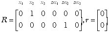
While one could drop variables to implement hypotheses such as
![]() =0,
the use of restricted least squares avoids recomputing the moment matrix (
=0,
the use of restricted least squares avoids recomputing the moment matrix (![]() ) and its inverse (
) and its inverse (![]() ), a
relatively lengthy task when n and k become large. In addition, restricted
least-squares can handle more general specifications such as the joint hypothesis
), a
relatively lengthy task when n and k become large. In addition, restricted
least-squares can handle more general specifications such as the joint hypothesis ![]() .
.
Sparsity and Computations
If differencing an observation with its nearby neighbors removes most of the effects of autocorrelation, the spatial weighting matrix D can be quite sparse. For example, if an observation displays error dependency with its nearest m neighbors, only m non-zero entries exist per row of D. Thus, D will contain nm non-zero elements out of n2 possible elements. This produces a m/n proportion of non-zero elements, a popular measure of sparsity. For example, with this problem we used four neighbors for each observation. Hence, D has sparsity of 4/3107 (0.13%). This represents a very high level of sparsity which increases as n grows.
Sparsity results in a number of computational gains. First, it dramatically decreases
the storage needed for D and ![]() . Using
traditional dense techniques, D requires 77.28MB of storage (double precision).
Using sparse matrix techniques, D requires less than 1MB of storage. Naturally,
this divergence grows with n. The use of sparse matrix technology has allowed us to
handle problems with 20,640 observations (Pace and Barry forthcoming).
. Using
traditional dense techniques, D requires 77.28MB of storage (double precision).
Using sparse matrix techniques, D requires less than 1MB of storage. Naturally,
this divergence grows with n. The use of sparse matrix technology has allowed us to
handle problems with 20,640 observations (Pace and Barry forthcoming).
Second, sparsity greatly accelerates computations. For example, multiplying the n
by n matrix D by the n by k matrix X requires O(kn2)
operations using dense matrices. Barring computational bookkeeping, the equivalent sparse
operation requires O(knm) operations. The real benefits come when computing
determinants, inverses, or solving systems of equations. All of these operations can build
upon the LU decomposition of a matrix through Gaussian elimination and all require O(n3)
operations when using dense matrices (Golub and Van Loan 1989). Sparsity, however, can
totally change the order of the number of operations required in these computations. For
example, if ![]() had a band structure with
lower bandwidth p and upper bandwidth q, the LU decomposition of
had a band structure with
lower bandwidth p and upper bandwidth q, the LU decomposition of ![]() , would require O(2npq) operations (Golub
and Van Loan 1989, p. 151). Hence, for fixed bandwidths the computations grow linearly
with n, the number of observations.
, would require O(2npq) operations (Golub
and Van Loan 1989, p. 151). Hence, for fixed bandwidths the computations grow linearly
with n, the number of observations.
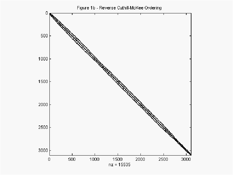
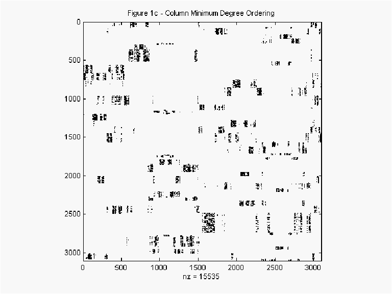
Unfortunately, the existence of a pure band structure does not arise very often. Figure
1a shows the actual plot of the non-zero elements in ![]() . Each of the blocks on the diagonals represent states. The dispersed
off-diagonal elements represent counties contiguous with those from a different state. The
existence of such dispersed off-diagonals could make it difficult to achieve computational
gains. However, one can permute the rows or columns of
. Each of the blocks on the diagonals represent states. The dispersed
off-diagonal elements represent counties contiguous with those from a different state. The
existence of such dispersed off-diagonals could make it difficult to achieve computational
gains. However, one can permute the rows or columns of ![]() using the reverse Cuthill-McKee algorithm to create a variable band matrix as
shown in Figure 1b. Figure 1b makes the gains of exploiting sparsity obvious. Less
obviously, Figure 1c shows the plot of
using the reverse Cuthill-McKee algorithm to create a variable band matrix as
shown in Figure 1b. Figure 1b makes the gains of exploiting sparsity obvious. Less
obviously, Figure 1c shows the plot of ![]() permuted using the column minimum degree algorithm. Counterintuitively, this ordering
usually produced the fastest LU decomposition times. See George and Liu (1981) for a
discussion of the reverse Cuthill-McKee, minimum degree, and other orderings useful in
accelerating the computation of matrix decompositions.
permuted using the column minimum degree algorithm. Counterintuitively, this ordering
usually produced the fastest LU decomposition times. See George and Liu (1981) for a
discussion of the reverse Cuthill-McKee, minimum degree, and other orderings useful in
accelerating the computation of matrix decompositions.
While the actual mechanics of these algorithms may seem quite involved, the intuition is simple. If one had many equations to solve, the fewer variables in each equation the better (more sparsity preferred). It seems intuitive to arrange the equations so that each one uses variables present only in nearby equations (low bandwidth preferred). Ideally, one would like to order the equations so that one could solve the first one for a variable, then take this variable’s value, substitute it into the second one, solve for the second variable, and so on. Gaussian elimination and the LU decomposition allow one to perform precisely this procedure. Hence, these algorithms formalize and swiftly execute a natural set of computations.
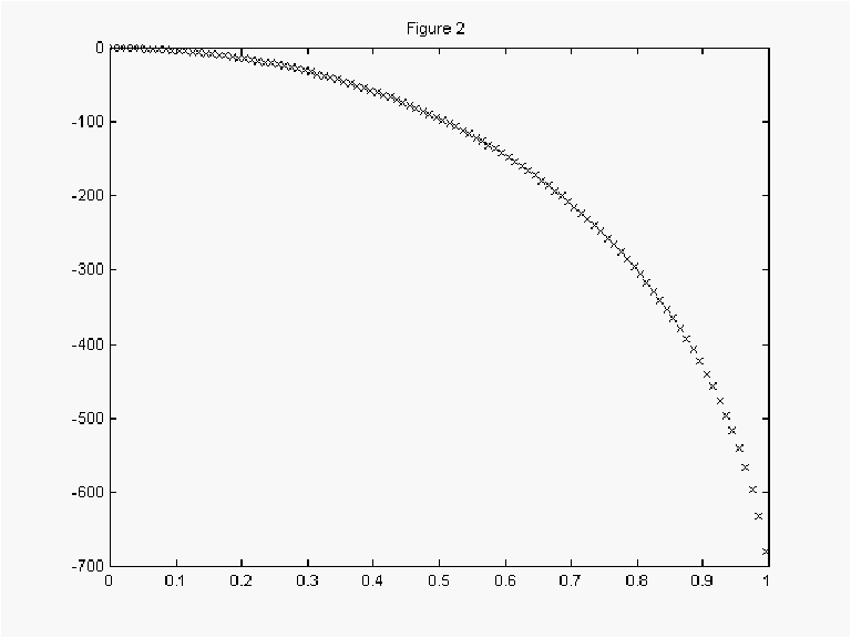
We computed ![]() for 100 values of a over [.005, .015, ... .995]. Figure 2 shows the plot of the
log-determinants versus a . Table 1 shows the timings
associated with computing the LU decomposition using the original, random, reverse
Cuthill-McKee, and column minimum degree orderings for
for 100 values of a over [.005, .015, ... .995]. Figure 2 shows the plot of the
log-determinants versus a . Table 1 shows the timings
associated with computing the LU decomposition using the original, random, reverse
Cuthill-McKee, and column minimum degree orderings for ![]() . As Table 1 makes clear, the ordering of the rows and columns matter, with
the column minimum degree ordering reducing execution times by 91.98% over the original
ordering. The column minimum degree ordering also reduced execution times by 58.71% over
the more intuitive reverse Cuthill-McKee ordering. As a worst case scenario, the random
ordering produced computational times worse than the optimal ordering by a factor of
105.95. All computations used the Matlab language running on a 200Mhz Pentium Pro
computer.
. As Table 1 makes clear, the ordering of the rows and columns matter, with
the column minimum degree ordering reducing execution times by 91.98% over the original
ordering. The column minimum degree ordering also reduced execution times by 58.71% over
the more intuitive reverse Cuthill-McKee ordering. As a worst case scenario, the random
ordering produced computational times worse than the optimal ordering by a factor of
105.95. All computations used the Matlab language running on a 200Mhz Pentium Pro
computer.
To place these results in perspective, Li (1995) took the eigenvalue route to computing determinants. Li used an IBM RS6000 Model 550 and a CM5 parallel processing supercomputer. The CM5 had 32 processors each with 32MB of local memory and four vector units. For a 2500 by 2500 spatial weight matrix the RS6000 required 8515.07 seconds while the CM5 required 45.78 seconds. Adjusting for size differences ((3107/2500)3) these times would go to 16345.26 and 87.88 seconds for a 3107 by 3107 problem. Hence, the use of sparse technology allows personal computers to approach supercomputer performance for this problem.
The use of sparsity does not preclude the use of supercomputing technology. A substantial amount of development has gone into devising parallel sparse routines (Saad 1996, p. 324-422). Employing supercomputers and sparseness could vastly extend the range of computable spatial problems. Moreover, as demonstrated herein, one can easily vectorize spatial estimators.
Note, the smoothness of ![]() suggests we could evaluate it over
fewer values of a or concentrate the computations around a likely to occur. We have achieved good performance with the use of
a 20th degree polynomial, which would reduce the number of determinant computations above
by a factor of five.
suggests we could evaluate it over
fewer values of a or concentrate the computations around a likely to occur. We have achieved good performance with the use of
a 20th degree polynomial, which would reduce the number of determinant computations above
by a factor of five.
Voting Across Counties
In this section we illustrate the techniques presented in previous sections using data on the votes cast in the 1980 presidential election across U.S. counties. In what follows, part 1 discusses the data employed, part 2 presents the two models used, part 3 gives the estimation results, while part 4 demonstrates the use of the likelihood ratio tests discussed in a previous section.
1. Voting Data
Specifically, we used the geographic centroids from all the counties (or their equivalents) in the continental U.S. from the 1990 Census which recorded votes in the 1980 presidential election. This yielded a matrix D with 3,107 rows and 3,107 columns. We picked 1980 because the presidential election cycle of every four years corresponded to the census data collection cycle of every ten years.
We collected data on the total number of votes cast in the 1980 presidential election per county (Votes), the population in each county of 18 years of age or older (Pop), the population in each county with a 12th grade or higher education (Education), the number of owner-occupied housing units (Houses), and the aggregate income (Income).
2. Models
We fitted two models by OLS and maximum likelihood, respectively. We elected to examine the log of the proportion of votes cast for both candidates in the 1980 presidential election. Hence, we can express our dependent variable as ln(PrVotes)= ln(Votes/ Pop) = ln(Votes)-ln(Pop). We fitted the following model via OLS:
ln(PrVotes)=Interceptb 1+ln(Pop)b 2+ln(Education)b 3+ln(Houses)b 4
+ln(Income)b 5+e
We fitted the following model which subsumes the previous model via maximum likelihood:
ln(PrVotes)=Interceptb 1+ln(Pop)b 2+ln(Education)b 3+ln(Houses)b 4
+ln(Income)b 5+Dln(Pop)b 6+Dln(Education)b 7+Dln(Houses)b 8
+Dln(Income)b 9+ Dln(PrVotes) a +e
This looks at the same fundamental model, but adds to it the spatial lags of the dependent and independent variables.
3. Estimation Results
As Table 2 documents, both the OLS and maximum likelihood predictions showed reasonably good relative fit with R2s of .5242 and .7123. As this indicates, maximum likelihood using the spatial information displayed considerably lower error than OLS. In fact, the SSE from OLS of 49.2825 was 78.12% higher than the SSE of 27.6686 from maximum likelihood. Moreover, the median absolute error from OLS of .0864 was 40.49% higher than the median absolute error of .0615 from maximum likelihood.
The OLS estimates displayed the expected signs with the exception of income which was negative and significant. The variable ln(Pop) had a negative sign for both OLS and maximum likelihood. However, this arises because we use the proportion of votes cast which effectively removes a coefficient of 1 from both sides. Given the measured coefficients on ln(Pop) were greater than -1, population has the expected positive overall effect on votes but the proportion voting declines with population per se. Similarly, maximum likelihood on the expanded model displayed the expected signs on all the variables. Inspection of the maximum likelihood results show the probable source of OLS’s difficulties. The significance of spatially lagged income, which the OLS model omits, and its correlation with income, led OLS to adjust towards the negative and significant omitted variable.
Relative to OLS, maximum likelihood ascribes a smaller influence of education and a larger influence of home ownership upon the propensity to vote. Naturally, the large coefficient on the lagged dependent variable suggests the existence of geographically correlated but omitted variables.
4. Inference
The second section discussed means of avoiding computation of the information matrix in a spatial setting. When the likelihood costs little to compute, likelihood ratio tests have substantial appeal. In this case, the restricted maximum likelihood estimates do not require much computational resources. We test the hypotheses that each of the basic independent variables and their spatial lags have no effect upon the regression. As we have nine total independent variables (four basic variables, four spatially lagged basic independent variables, and an intercept), the matrix R has 4 rows and 9 columns. It contains all zeros except for a one in each row in the position of the variables whose effects we wish to set to zero. The vector r is a 4 by 1 vector of zeros.
Table 3 displays the results of the likelihood ratio tests for the deletion of all spatially lagged variables, of the spatially lagged dependent variable, and all of the basic independent variables with their lags. All of the variables or combinations of the variables were statistically significant. It required only .09 seconds to compute the restricted likelihoods for the deletion of the basic independent variables with their lags using the techniques presented earlier.
The likelihood associated with the OLS regression on the basic variables coupled with the maximum likelihood obtained for all variables give the likelihood ratio test for the significance of all spatially lagged variables. The likelihood associated with a =0 from the profile likelihood coupled with the maximum likelihood for all variables obtained give the likelihood ratio test for the significance of the spatially lagged dependent variable, Dy. These likelihoods require no additional computations but appear as a byproduct from the basic procedure and hence impose little computational cost.
The significance of a , the parameter estimate of the spatially lagged dependent variable, and the significance of the other spatially lagged independent variables shows the substantial contribution geographically correlated variables make to the overall fit.
An Illustrative Simulation
This section examines a simulation of 22,500 regressions each using 3107 observations. Part 1 discusses the data, part 2 gives the timings of the simulation computations, and part 3 provides the statistical results.
1. Simulation Data
To provide verisimilitude to the simulation, we chose the same spatial weighting matrix as employed in the empirical voting example.
In the simulation, we:
1. Generated uniform random variables for nine columns of X and used a constant for the other column.
2. Set b to a vector of ones.
3. Let a v equal [.01, .05, .1, .25, .5, .75, .9, .95, .99].
4. Set s to each of [.1, .5, 1, 2, 10].
5. Generated a common set of 250 N(0,1) vectors of 3107 elements each using the Matlab normal random number generator. We perform this operation once for the entire simulation. Scaling the common N(0,1) errors by s generates the N(0, s 2) random variables. This practice, referred to as "correlated sampling" (Rubinstein (1981)) greatly reduces the variance in Monte Carlo experiments.
We subsequently generated the autocorrelated dependent variable, y, according to ,
![]()
()15
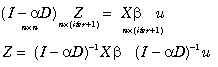
where u represents an n by iter matrix of N(0,1) random variates where iter represents the number of iterations in the experiment. In actuality, we solved the corresponding equation system in for the coefficients Z via Gaussian elimination using an LU decomposition rather than computing the inverse as this goes much faster.
()16
Compare this to the usual inverse formulation,

()17
Relative to , requires solving a larger system (n by n instead of n by (iter+1)) and subsequently multiplying an n by n matrix by a n by iter +1 matrix (O(n2(iter+1))). Since iter+1 usually is much smaller than n, the inverse method takes substantially longer to yield the same results.
2. Timing Results from the Monte Carlo Experiment
Table 4 contains the results from the Monte Carlo experiment using the autoregressive dependent variable model. Table 4 contains 45 cases resulting from nine autoregressive parameter values, a , and five levels of error variability, s . Each case contains the average of the results from five runs of 100 iterations each. The runs required 36.8 minutes in total. Thus, each maximum likelihood spatial autoregression and simulated dependent variable needed 0.1 seconds of computational time, a very low figure.
3. Statistical Results from the Monte Carlo Experiment
The results in Table 4 match some of those reported in the literature using regular lattices. First, the maximum likelihood estimator slightly underestimates the true differencing parameter, a . Second, the EGLS estimator overestimates a . Note, two versions of the EGLS estimator appear. The first one comes from . The second one comes from picking the value of a off the grid which minimizes SSE. Hence, one could consider EGLS2 an inequality restricted EGLS estimator. It has the same granularity problem as the maximum likelihood estimator and hence makes a better comparison with the maximum likelihood estimator. For example, examine the cases where a equals 0.99. In these cases, both the EGLS2 and ML give the same value of the square root of the mean squared error (RMSE) of 0.05. However, as the comparison between EGLS1 and EGLS2 reveals, for most cases the granularity problem does not greatly affect the results. The inequality restricted nature of EGLS2 does lead to it performing differently than EGLS1 at the endpoints.
Third, the maximum likelihood estimator greatly outperforms EGLS in most cases. In fact, maximum likelihood displays a factor of 14.81 better performance at the worst case for EGLS (a =.5, s =10). EGLS becomes most acceptable for high a and low s . Fourth, all of the estimators perform worse as s rises.
Each estimator reaches the nadir of its performance at various points depending upon both a and s . For example, the maximum likelihood estimator reaches its nadir at a of 0.1 with s of 10. The EGLS1 estimator reaches its nadir at a of 0.5 with s of 10.
Conclusion
A variety of methods can greatly accelerate the computation of large scale spatial autoregressions. This paper explored the use of sparse matrix techniques, formulating the profile likelihood to avoid iterative computations, and using restricted least squares to form likelihood ratio tests as opposed to computing information matrices. As illustrations of the efficacy of these techniques, we looked at an empirical example at the county level and conducted a Monte Carlo experiment with 22,500 spatial autoregressions. Despite the formidable size of the regressions (3107 observations), these cost only 0.1 seconds each to generate the spatially dependent variable and estimate the coefficients.
The voting example showed the power of geographic information to help clarify social phenomenon. OLS on the non-spatial variables displayed 78% higher sum-of-squared errors than maximum likelihood on the combination of spatial and non-spatial variables. Relative to OLS, maximum likelihood ascribes a smaller influence of education and a larger influence of home ownership upon the propensity to vote. More importantly, OLS shows income has a significant, negative effect on the proportion voting while maximum likelihood shows income has a small positive but statistically insignificant effect. However, spatially lagged income has a significant, negative effect upon voting.
Hopefully, additions like these to the spatial statistics toolkit will allow computations to keep pace with the ever-increasing flow of geographic information and bring spatial techniques into more routine usage.
Literature Cited
Anselin, L. (1988). Spatial Econometrics: Methods and Models. Dordrecht: Kluwer.
Anselin, L., and S. Hudak (1992). "Spatial Econometrics in Practice: A Review of Software Options." Journal of Regional Science and Urban Economics 22, 509-536.
Bureau of the Census, USA Counties on CD-Rom, 1994.
Can, A. (1992). "Specification and Estimation of Hedonic Housing Price Models." Regional Science and Urban Economics 22, 453-474.
Can, A., and I. Megbolugbe (forthcoming). "Spatial Dependence and House Price Index Construction." Journal of the Real Estate Finance and Economics.
Cressie, N. (1993). Statistics for Spatial Data. Revised ed. New York: John Wiley.
Dubin, R. (1988). "Spatial Autocorrelation." Review of Economics and Statistics 70, 466-474.
George, A., and J. Liu (1981). Computer Solution of Large Sparse Positive Definite Systems. Englewood Cliffs: Prentice-Hall.
Gilley, O., and K. Pace (1995). "Using Inequality Restrictions to Tame Multicollinearity in Hedonic Pricing Models." Review of Economics and Statistics 77, 609-621.
Golub, G., and C. Van Loan (1989). Matrix Computations. Second ed. Baltimore: John Hopkins.
Griffith, D. (1988). "Estimating Spatial Autoregressive Model Parameters with Commercial Statistical Software." Geographical Analysis 20, 176-186.
Griffith, D. (1995). "Some Guidelines for Specifying the Geographic Weights Matrix Contained in Spatial Statistical Models," in: Arlinghaus, S., ed. Practical Handbook of Spatial Statistics. Boca Raton: CRC Press, 65-82.
Haining, R. (1990). Spatial Data Analysis in the Social and Environmental Sciences. Cambridge: Cambridge University Press.
Judge, et al. (1988). Introduction to the Theory and Practice of Econometrics. New York: John Wiley.
Li, B. (1995). "Implementing Spatial Statistics on Parallel Computers," in: Arlinghaus, S., ed. Practical Handbook of Spatial Statistics. Boca Raton: CRC Press, 107-148.
Meeker, W., and L. Escobar (1995). "Teaching about Approximate Confidence Regions Based on Maximum Likelihood Estimates." The American Statistician 49, 48-53.
Ord, K. (1975). "Estimation Methods for Models of Spatial Interaction." Journal of the American Statistical Association 70, 120-126.
Pace, K., and R. Barry (forthcoming). "Sparse Spatial Autoregressions." Statistics and Probability Letters.
Pace, K., and O. Gilley (forthcoming). "Using the Spatial Configuration of the Data to Improve Estimation." Journal of the Real Estate Finance and Economics.
Pace, K. and O. Gilley (1993). "Improving Prediction and Assessing Specification Quality in Non-Linear Statistical Valuation Models." Journal of Business and Economics Statistics 11, 301-310.
Ripley, B. (1981). Spatial Statistics. New York: John Wiley.
Ripley, B. (1988). Statistical Inference for Spatial Processes. Cambridge: Cambridge University Press.
Rubinstein, R. (1981). Simulation and the Monte Carlo Method. New York: John Wiley.
Saad, Y. (1996). Iterative Methods for Sparse Linear Systems. Boston: PWS Publishing.
| Table 1 — Execution Times in Seconds Versus Ordering Algorithm |
||
| Ordering Algorithm | LU |
|
| Original | 10.35 | |
| Reverse Cuthill-McKee | 2.01 | |
| Column Minimum Degree | 0.83 | |
| Random | 87.94 | |
Table 2 — OLS and ML Estimates of Voting Characteristics |
||||
Bols |
tols |
Bml |
tml |
|
| Intercept | 0.9814 | 20.9680 |
0.4582 |
10.2893 |
| ln(Population > 18 years of Age) | -0.8464 | -38.3780 |
-0.7174 |
-31.3059 |
| ln(Population with Education > 12 years) | 0.5167 | 33.4241 |
0.1910 |
8.1971 |
| ln(Owner Occupied Housing Units) | 0.4291 | 24.0222 |
0.4513 |
28.8363 |
| ln(Aggregate Income) | -0.1439 | -7.2680 |
0.0266 |
1.2089 |
| Lagged ln(Population > 18 years of Age) | 0.3999 |
-13.2999 |
||
| Lagged ln(Population with Education > 12 years) | 0.0513 |
1.9398 |
||
| Lagged ln(Owner Occupied Housing Units) | -0.2906 |
-12.9525 |
||
| Lagged ln(Aggregate Income) | -0.1252 |
-4.5015 |
||
| Optimal a | 0.6150 |
|||
| R2 | 0.5242 |
0.7123 |
||
| SSE | 49.2825 |
27.6686 |
||
| Median |e| | 0.0864 |
0.0615 |
||
| Log(Likelihood) | -6307.1 |
-5679.1 |
||
| n | 3107 |
3107 |
||
| k | 5 |
10 |
||
| Time | .03 sec |
.09 sec |
||
Table 3 — Likelihood Ratio Tests for the Deletion of Different Variables |
||||
| Deletion of: | Unrestricted Likelihood | Restricted Likelihood | Likelihood Ratio | Number of Hypotheses |
| All Spatially Lagged Variables | -5679.0911 | -6307.0766 | 1255.9710 | 5 |
| Dy | -5679.0911 | -6222.4552 | 1086.7282 | 1 |
| ln(Population > 18 years of Age) | -5679.0911 | -6120.5844 | 882.9866 | 2 |
| ln(Population with Education > 12 years) | -5679.0911 | -5809.8701 | 261.5580 | 2 |
| ln(Owner Occupied Housing Units) | -5679.0911 | -6045.2873 | 732.3924 | 2 |
| ln(Aggregate Income) | -5679.0911 | -5692.6655 | 27.1488 | 2 |
| Table 4 — True Vs. Estimated Parameters and RMSEs Across 500 Autoregressions | |||||||
|
|
|
|
|
|
|
||
| 0.01 | 0.1 | 0.0104 | 0.0105 | 0.0102 | 0.0051 | 0.0052 | 0.0042 |
| 0.01 | 0.5 | 0.0140 | 0.0172 | 0.0121 | 0.0116 | 0.0154 | 0.0201 |
| 0.01 | 1.0 | 0.0165 | 0.0236 | 0.0140 | 0.0155 | 0.0253 | 0.0336 |
| 0.01 | 2.0 | 0.0174 | 0.0284 | 0.0153 | 0.0172 | 0.0330 | 0.0438 |
| 0.01 | 10.0 | 0.0175 | 0.0307 | 0.0158 | 0.0179 | 0.0375 | 0.0493 |
| 0.05 | 0.1 | 0.0503 | 0.0510 | 0.0507 | 0.0053 | 0.0053 | 0.0042 |
| 0.05 | 0.5 | 0.0497 | 0.0605 | 0.0605 | 0.0163 | 0.0226 | 0.0223 |
| 0.05 | 1.0 | 0.0496 | 0.0733 | 0.0731 | 0.0220 | 0.0398 | 0.0401 |
| 0.05 | 2.0 | 0.0493 | 0.0841 | 0.0835 | 0.0244 | 0.0537 | 0.0542 |
| 0.05 | 10.0 | 0.0493 | 0.0896 | 0.0889 | 0.0252 | 0.0610 | 0.0617 |
| 0.10 | 0.1 | 0.1002 | 0.1013 | 0.1012 | 0.0053 | 0.0053 | 0.0043 |
| 0.10 | 0.5 | 0.0996 | 0.1209 | 0.1207 | 0.0160 | 0.0285 | 0.0282 |
| 0.10 | 1.0 | 0.0993 | 0.1462 | 0.1464 | 0.0222 | 0.0561 | 0.0563 |
| 0.10 | 2.0 | 0.0987 | 0.1674 | 0.1677 | 0.0249 | 0.0790 | 0.0792 |
| 0.10 | 10.0 | 0.0986 | 0.1791 | 0.1791 | 0.0259 | 0.0917 | 0.0917 |
| 0.25 | 0.1 | 0.2503 | 0.2528 | 0.2527 | 0.0052 | 0.0056 | 0.0047 |
| 0.25 | 0.5 | 0.2494 | 0.2982 | 0.2983 | 0.0154 | 0.0513 | 0.0514 |
| 0.25 | 1.0 | 0.2491 | 0.3594 | 0.3591 | 0.0205 | 0.1130 | 0.1127 |
| 0.25 | 2.0 | 0.2487 | 0.4093 | 0.4094 | 0.0234 | 0.1632 | 0.1634 |
| 0.25 | 10.0 | 0.2483 | 0.4367 | 0.4368 | 0.0245 | 0.1910 | 0.1910 |
| 0.50 | 0.1 | 0.5001 | 0.5043 | 0.5041 | 0.0050 | 0.0056 | 0.0052 |
| 0.50 | 0.5 | 0.4997 | 0.5771 | 0.5771 | 0.0129 | 0.0782 | 0.0782 |
| 0.50 | 1.0 | 0.4988 | 0.6731 | 0.6731 | 0.0170 | 0.1742 | 0.1742 |
| 0.50 | 2.0 | 0.4984 | 0.7514 | 0.7514 | 0.0192 | 0.2525 | 0.2525 |
| 0.50 | 10.0 | 0.4980 | 0.7940 | 0.7937 | 0.0199 | 0.2951 | 0.2948 |
| 0.75 | 0.1 | 0.7500 | 0.7546 | 0.7537 | 0.0050 | 0.0050 | 0.0043 |
| 0.75 | 0.5 | 0.7494 | 0.8197 | 0.8197 | 0.0088 | 0.0702 | 0.0701 |
| 0.75 | 1.0 | 0.7487 | 0.9055 | 0.9054 | 0.0114 | 0.1559 | 0.1558 |
| 0.75 | 2.0 | 0.7482 | 0.9738 | 0.9742 | 0.0128 | 0.2241 | 0.2245 |
| 0.75 | 10.0 | 0.7483 | 0.9944 | 1.0109 | 0.0135 | 0.2445 | 0.2612 |
| 0.90 | 0.1 | 0.9000 | 0.9046 | 0.9021 | 0.0050 | 0.0050 | 0.0023 |
| 0.90 | 0.5 | 0.8993 | 0.9388 | 0.9387 | 0.0056 | 0.0391 | 0.0388 |
| 0.90 | 1.0 | 0.8992 | 0.9864 | 0.9865 | 0.0067 | 0.0866 | 0.0866 |
| 0.90 | 2.0 | 0.8988 | 0.9950 | 1.0248 | 0.0074 | 0.0950 | 0.1250 |
| 0.90 | 10.0 | 0.8988 | 0.9950 | 1.0453 | 0.0077 | 0.0950 | 0.1455 |
| 0.95 | 0.1 | 0.9498 | 0.9545 | 0.9511 | 0.0050 | 0.0050 | 0.0013 |
| 0.95 | 0.5 | 0.9493 | 0.9727 | 0.9717 | 0.0050 | 0.0231 | 0.0218 |
| 0.95 | 1.0 | 0.9492 | 0.9949 | 0.9987 | 0.0052 | 0.0449 | 0.0488 |
| 0.95 | 2.0 | 0.9491 | 0.9950 | 1.0204 | 0.0054 | 0.0450 | 0.0707 |
| 0.95 | 10.0 | 0.9488 | 0.9950 | 1.0320 | 0.0056 | 0.0450 | 0.0823 |
| 0.99 | 0.1 | 0.9890 | 0.9935 | 0.9902 | 0.0050 | 0.0050 | 0.0003 |
| 0.99 | 0.5 | 0.9888 | 0.9950 | 0.9945 | 0.0050 | 0.0050 | 0.0046 |
| 0.99 | 1.0 | 0.9883 | 0.9950 | 0.9998 | 0.0050 | 0.0050 | 0.0100 |
| 0.99 | 2.0 | 0.9885 | 0.9950 | 1.0038 | 0.0050 | 0.0050 | 0.0141 |
| 0.99 | 10.0 | 0.9883 | 0.9950 | 1.0059 | 0.0050 | 0.0050 | 0.0162 |